These dynamic splats run backwards, and the round trip loses 1.3%
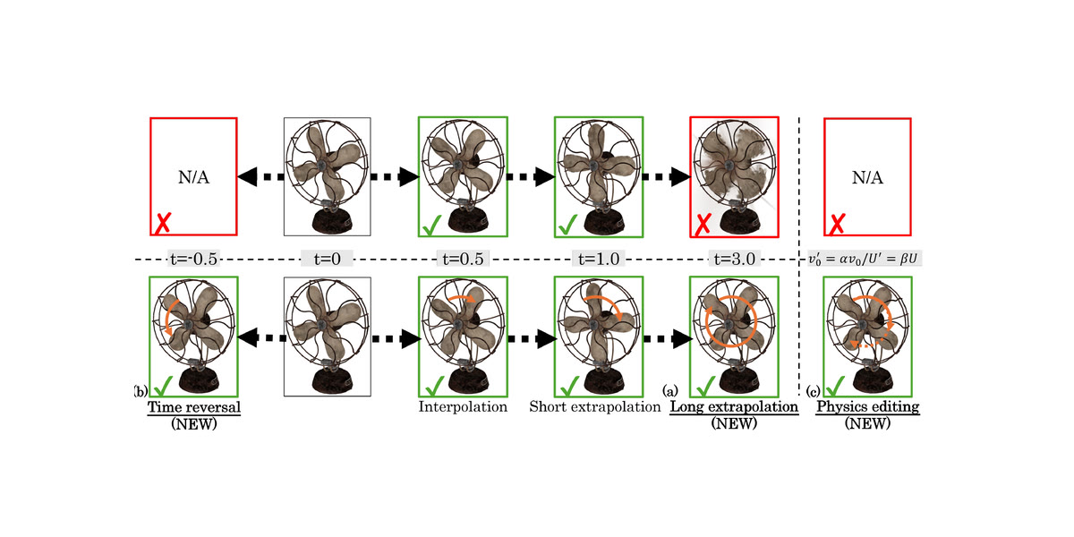
Figure: Sato et al., NTT (CC BY 4.0) · Research

Aug 26, 2026, 5:40 AM ETResearch
Shogo Sato and colleagues at NTT's Human Informatics Laboratories have published LagrangeGS, which takes the physics-aware dynamic splatting methods of the past two years and asks what happens if the motion is made to satisfy mechanics rather than merely resemble it. The answer is that you gain the ability to integrate the scene backwards in time, you stop objects inflating during long rollouts, and on the best available backbone your rendering metrics get worse.
Why it matters: Dynamic 3D Gaussian splatting reconstructs a moving scene beautifully inside the window it was trained on. Step outside that window and it falls apart, which is why a run of recent work has bolted physics onto it — usually by predicting a velocity field for the Gaussians and integrating forward.
LagrangeGS's argument is that predicting a velocity field is not physics. Those methods fit a vector field to observed visual deformation; nothing constrains the result to be a trajectory any mechanical system could actually follow. The paper lists three consequences: trajectories that are physically inconsistent, no time-reversibility, and geometric collapse when extrapolation runs long.
The fix is to write the whole thing as a non-conservative Lagrangian system — a potential energy, an initial velocity field, and a set of non-conservative forces — and let the mechanics generate the motion.
What they built: Applying a Lagrangian neural network directly to dynamic splatting is not tractable: it requires inverting a velocity-Hessian across millions of Gaussian particles. The authors approximate that Hessian as the identity, which decouples the particles from one another and makes the whole thing solvable. It is a large approximation and they say so.
Time-reversibility falls out of a second restriction. If the non-conservative forces are constrained to be explicitly time-independent, the same trained network can be integrated backward with a negative timestep and recover past states. This is the part that is genuinely new — not replaying stored frames in reverse, but computing what the scene was doing before the capture started.
The third problem, geometric collapse, gets a local rigid alignment term that regularises particle trajectories against their neighbours.
By the numbers:
- Applied to DefGS, LagrangeGS adds 5.05 dB on the Dynamic Object benchmark (19.85 to 24.90) and 9.99 dB on Dynamic Indoor Scene (21.38 to 31.37).
- Applied to FreeGave, it subtracts 3.05 dB and 1.92 dB respectively. FreeGave alone scores 31.99 and 35.02; the strongest prior baseline, TRACE, scores 31.60 and 34.82.
- Backward integration is close to exact: the mean cycle error over a forward-and-back rollout is 1.3% on Dynamic Object and 0.19% on Dynamic Indoor Scene, and the per-particle velocity vectors invert cleanly across t = 0.
- On long rollouts LagrangeGS stays within 1.1× its initial foreground extent. FreeGave expands to 1.9× — the collapse mode the method exists to prevent.
- Truncate the training window and the ranking flips. At t < 0.3 on Dynamic Object, LagrangeGS beats FreeGave by 0.91 dB (22.27 against 21.34), having trailed it by 3.05 dB on the full window.
Yes, but: The FreeGave regression is the paper's most interesting passage, because rather than bury it the authors went looking for where the decibels went. Their hypothesis is that strict physical regularisation prunes visual artefacts that are not physical — shadows, primarily — and that a shadow you refuse to render is a shadow the ground truth still contains.
To test that they recomputed PSNR on binarised foreground silhouettes, which discards appearance and keeps shape. On Dynamic Object the gap was unchanged, −3.2 dB in both RGB and silhouette, meaning the loss there really is geometric. On Dynamic Indoor Scene it collapsed from −2.5 dB to −0.6 dB, meaning that loss was almost entirely appearance — moving shadows, as predicted.
So one of the two regressions is explained and one is not. That is a more useful result than a clean win would have been, and the truncation experiment gives it a shape: the physics prior is a cost when observations are dense and a benefit when they are sparse. It is a regulariser, and it behaves like one.
The identity approximation on the velocity-Hessian remains unexamined. Decoupling particle dynamics is what makes the method run, and it also means the particles cannot exert force on each other — which is a strange thing for a mechanical system to be unable to do.
The big picture: Time reversal is the capability worth watching here, and not because anyone urgently needs to see a fan spin backwards. It is a test that is hard to fake. A model that has learned an animation shortcut cannot integrate backwards and land where it started; a model that has learned continuous mechanics can. A 1.3% cycle error is evidence about what was learned, not just about what can be rendered.
The counterfactual editing follows from the same property. Scale the initial velocity, change the force parameters, and the scene replays under different physics without retraining — because the physics was a parameter of the representation rather than a pattern fitted to the pixels.